AI绘画：什么是Diffusion模型

这是一篇关于 What are Diffusion Models 的译文。很多地方借鉴了由浅入深了解Diffusion Model 一文。

2022年最火的AI算法要属AIGC：（AI-generated content，AI生成内容）。这一概念最开始是由OpenAI推出的DALL·E模型进入到大家的视野。DALL·E算法模型可以根据一段文本生成一张和文本相关的图片，所以这种模型也被称作Text2Image模型。

而随着更多组织，专业人士加入研究AIGC行列，Text2Image算法模型的生成质量也被不断提高。像Open AI推出的DALL·E-2, Google的 Imagen 和 Parti，国内的百度文心，都可以生成非常高质量的图像。但上述几个模型并不开源，且申请licence也比较困难（OpenAI会直接reject香港IP的申请），所以能够体验到的人也很少。

但随着开源项目Stable Diffusion的release，人们可以免费使用这个模型，并且更重要的是，开发者，研究者可以在此基础上做二次的模型优化和研发。随着Stable Diffusion 的public release,关于AI绘画的应用和讨论也变得越来越多，越来越多的圈外人士对这一技术产生了兴趣。

本文主要介绍什么是DDPM：Denoising Diffusion Probabilistic Models(DDPM; Ho et al. 2020).

Basic Knowledge

Normal Distribution: $$\mathcal{N}(x; \mu, \sigma^2) = \frac{1}{\sqrt{2\pi}\sigma} \exp \left( -\frac{(x - \mu)^2}{2\sigma^2} \right)$$
Conditional Probability: $${\displaystyle P(A\mid B)={\frac {P(A\cap B)}{P(B)}}}$$
Bayes’ theorem: $${\displaystyle P(A\mid B)={{P(B\mid A)P(A)} \over {P(B)}}}$$
KL divergence: $$D_{\text{KL}}(q(x) || p(x)) = \mathbb{E}_{q(x)} \log [q(x) / p(x)]$$

DDPM

Forward diffusion process

从给定的真实数据集中采样一个数据样本：${x}_0 \sim q({x})$; 在前向扩散过程中，我们逐步向样本中添加少量高斯噪声，产生一系列噪声样本: ${x}_1,\dots,{x}_T$;步长 $t$ 由方差控制 ${\beta_t\in (0, 1)}_{t=1}^T$

随着步长$t$的变大，数据样本$\mathbf{x}_0$逐渐失去其自身特征。最终，当$T\to\infty$ , $\mathbf{x}_T$等价于各向同性高斯分布。

Untitled

上述过程有一个很好的特性，我们可以使用重参数化技巧以封闭形式在任意时间步$t$采样$\mathbf{x}_t$。

定义 $\alpha_t = 1 - \beta_t$ and $\bar{\alpha}_t = \prod_{i=1}^t \alpha_i$

$$\begin{aligned} \mathbf{x}_t &= \sqrt{\alpha_t}\mathbf{x}_{t-1} + \sqrt{1 - \alpha_t}\boldsymbol{\epsilon}_{t-1} & \text{ ;where } \boldsymbol{\epsilon}_{t-1}, \boldsymbol{\epsilon}_{t-2}, \dots \sim \mathcal{N}(\mathbf{0}, \mathbf{I}) \\ &= \sqrt{\alpha_t \alpha_{t-1}} \mathbf{x}_{t-2} + \sqrt{1 - \alpha_t \alpha_{t-1}} \bar{\boldsymbol{\epsilon}}_{t-2} & \text{ ;where } \bar{\boldsymbol{\epsilon}}_{t-2} \text{ merges two Gaussians (*).} \\ &= \dots \\ &= \sqrt{\bar{\alpha}_t}\mathbf{x}_0 + \sqrt{1 - \bar{\alpha}_t}\boldsymbol{\epsilon} \\ q(\mathbf{x}_t \vert \mathbf{x}_0) &= \mathcal{N}(\mathbf{x}_t; \sqrt{\bar{\alpha}_t} \mathbf{x}_0, (1 - \bar{\alpha}_t)\mathbf{I}) \end{aligned}$$

(*) 合并两个高斯分布 $\mathcal{N}(\mathbf{0}, \sigma_1^2\mathbf{I})$和 $\mathcal{N}(\mathbf{0}, \sigma_2^2\mathbf{I})$，得到的新的高斯分布是$\mathcal{N}(\mathbf{0},(\sigma_1^2 + \sigma_2^2)\mathbf{I})$，合并后的标准差是：$\sqrt{(1 - \alpha_t) + \alpha_t (1-\alpha_{t-1})} = \sqrt{1 - \alpha_t\alpha_{t-1}}$

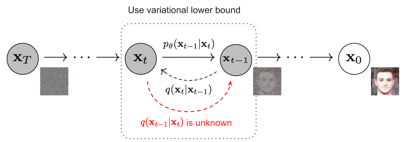
Reverse diffusion process

前向过程是扩散（加噪）过程，逆向过程就是去噪。如果我们可以反转扩散过程，得到逆转后的分布 $q(\mathbf{x}_{t-1} \vert \mathbf{x}_t)$ ，就可以从标准高斯分布 $\mathbf{x}_T \sim \mathcal{N}(\mathbf{0}, \mathbf{I})$ 中还原出原图分布$\mathbf{x}_0$。

如果$\beta_t$足够小的话，$q(\mathbf{x}_{t-1} \vert \mathbf{x}_t)$也是高斯分布。

不过我们无法简单得到 $q(\mathbf{x}_{t-1} \vert \mathbf{x}_t)$。因此我们使用深度学习模型 $p_\theta$ 来预测这样一个逆向分布。

$p_\theta(\mathbf{x}_{0:T}) = p(\mathbf{x}_T) \prod^T_{t=1} p_\theta(\mathbf{x}_{t-1} \vert \mathbf{x}_t) \quad$

$p_\theta(\mathbf{x}_{t-1} \vert \mathbf{x}_t) = \mathcal{N}(\mathbf{x}_{t-1}; \boldsymbol{\mu}_\theta(\mathbf{x}_t, t), \boldsymbol{\Sigma}_\theta(\mathbf{x}_t, t))$

我们无法得到逆向后的分布 $q(\mathbf{x}_{t-1} \vert \mathbf{x}_t)$，但如果知道$\mathbf{x}_0$，是可以通过贝叶斯公式得到$q(\mathbf{x}_{t-1} \vert \mathbf{x}_t, \mathbf{x}_0)$为：

$q(\mathbf{x}_{t-1} \vert \mathbf{x}_t, \mathbf{x}_0) = \mathcal{N}(\mathbf{x}_{t-1}; \color{blue}{\tilde{\boldsymbol{\mu}}}(\mathbf{x}_t, \mathbf{x}_0), \color{red}{\tilde{\beta}_t} \mathbf{I})$

具体的推导如下： $$\begin{aligned} q(\mathbf{x}_{t-1} \vert \mathbf{x}_t, \mathbf{x}_0) &= q(\mathbf{x}_t \vert \mathbf{x}_{t-1}, \mathbf{x}_0) \frac{ q(\mathbf{x}_{t-1} \vert \mathbf{x}_0) }{ q(\mathbf{x}_t \vert \mathbf{x}_0) } \\ &\propto \exp \Big(-\frac{1}{2} \big(\frac{(\mathbf{x}t - \sqrt{\alpha_t} \mathbf{x}_{t-1})^2}{\beta_t} + \frac{(\mathbf{x}_{t-1} - \sqrt{\bar{\alpha}_{t-1}} \mathbf{x}_0)^2}{1-\bar{\alpha}_{t-1}} - \frac{(\mathbf{x}_t - \sqrt{\bar{\alpha}_t} \mathbf{x} _0)^2}{1-\bar{\alpha}_t} \big) \Big) \\ &= \exp \Big(-\frac{1}{2} \big(\frac{\mathbf{x}t^2 - 2\sqrt{\alpha_t} \mathbf{x}_t \color{blue}{\mathbf{x}_{t-1}} \color{black}{+ \alpha_t} \color{red}{\mathbf{x}_{t-1}^2} }{\beta_t} + \frac{ \color{red}{\mathbf{x}_{t-1}^2} \color{black}{- 2 \sqrt{\bar{\alpha}_{t-1}} \mathbf{x}_0} \color{blue}{\mathbf{x}_{t-1}} \color{black}{+ \bar{\alpha}_{t-1} \mathbf{x}_0^2} }{1-\bar{\alpha}_{t-1}} - \frac{(\mathbf{x}_t - \sqrt{\bar{\alpha}_t} \mathbf{x}_0)^2}{1-\bar{\alpha}_t} \big) \Big) \\ &= \exp\Big( -\frac{1}{2} \big( \color{red}{(\frac{\alpha_t}{\beta_t} + \frac{1}{1 - \bar{\alpha}_{t-1}})} \mathbf{x}_{t-1}^2 - \color{blue}{(\frac{2\sqrt{\alpha_t}}{\beta_t} \mathbf{x}_t + \frac{2\sqrt{\bar{\alpha}_{t-1}}}{1 - \bar{\alpha}_{t-1}} \mathbf{x}_0)} \mathbf{x}_{t-1} \color{black}{ + C(\mathbf{x}_t, \mathbf{x}_0) \big) \Big)} \end{aligned}$$

其中第一步贝叶斯公式部分：

$q(x_{t-1}|x_t, x_0) = q(x_t|x_{t-1}, x_0) \frac{q(x_{t-1}|x_0)}{q(x_{t}| x_0)}$

$P(A \mid B,C) = \frac{P(B \mid A,C) ; P(A \mid C)}{P(B \mid C)}$

Proof:

$\begin{aligned} P(A\mid B, C) & = \frac{P(A,B,C)}{P(B, C)} \\ & =\frac{P(B\mid A,C),P(A, C)}{P(B, C)} \\ & =\frac{P(B\mid A,C),P(A\mid C),P(C)}{P(B, C)} \\ & =\frac{P(B\mid A,C),P(A\mid C) P(C)}{P(B\mid C) P(C)} \\ & =\frac{P(B\mid A,C);P(A\mid C)}{P(B\mid C)} \end{aligned}$

一般的高斯密度函数的指数部分应该写为：

Untitled

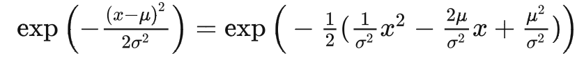
其中 $C(\mathbf{x}_t, \mathbf{x}_0)$是与$\mathbf{x}_{t-1}$ 无关的常数项。按照标准高斯密度函数，均值和方差可以参数化如下（回想一下 $\alpha_t = 1 - \beta_t$ 和 $\bar{\alpha}_t = \prod_{i=1}^T \alpha_i$):

$$\begin{aligned} \tilde{\beta}t &= 1/(\frac{\alpha_t}{\beta_t} + \frac{1}{1 - \bar{\alpha}_{t-1}}) = 1/(\frac{\alpha_t - \bar{\alpha}_t + \beta_t}{\beta_t(1 - \bar{\alpha}_{t-1})}) = \color{green}{\frac{1 - \bar{\alpha}_{t-1}}{1 - \bar{\alpha}_t} \cdot \beta_t} \\ \tilde{\boldsymbol{\mu}}_t (\mathbf{x}_t, \mathbf{x}_0) &= (\frac{\sqrt{\alpha_t}}{\beta_t} \mathbf{x}_t + \frac{\sqrt{\bar{\alpha}_{t-1} }}{1 - \bar{\alpha}_{t-1}} \mathbf{x}0)/(\frac{\alpha_t}{\beta_t} + \frac{1}{1 - \bar{\alpha}_{t-1}}) \\ &= (\frac{\sqrt{\alpha_t}}{\beta_t} \mathbf{x}_t + \frac{\sqrt{\bar{\alpha}_{t-1} }}{1 - \bar{\alpha}_{t-1}} \mathbf{x}0) \color{green}{\frac{1 - \bar{\alpha}_{t-1}}{1 - \bar{\alpha}_t} \cdot \beta_t} \\ &= \frac{\sqrt{\alpha_t}(1 - \bar{\alpha}_{t-1})}{1 - \bar{\alpha}_t} \mathbf{x}_t + \frac{\sqrt{\bar{\alpha}_{t-1}}\beta_t}{1 - \bar{\alpha}_t} \mathbf{x}_0\\ \end{aligned}$$

因为：

$\begin{aligned} \mathbf{x}_t&=\sqrt{\bar{\alpha}_t}\mathbf{x}_0 + \sqrt{1 -\bar{\alpha}_t}\boldsymbol{\epsilon} \ \end{aligned}$

可以整理成：

$\mathbf{x}_0 = \frac{1}{\sqrt{\bar{\alpha}_t}}(\mathbf{x}_t - \sqrt{1 - \bar{\alpha}_t}\boldsymbol{\epsilon}_t)$

把它带入上述方程得到：

$$\begin{aligned} \tilde{\boldsymbol{\mu}}_t &= \frac{\sqrt{\alpha_t}(1 - \bar{\alpha}_{t-1})}{1 - \bar{\alpha}_t} \mathbf{x}_t + \frac{\sqrt{\bar{\alpha}_{t-1}}\beta_t}{1 - \bar{\alpha}_t} \frac{1}{\sqrt{\bar{\alpha}_t}}(\mathbf{x}_t - \sqrt{1 - \bar{\alpha}_t}\boldsymbol{\epsilon}_t) \\ &= \color{cyan}{\frac{1}{\sqrt{\alpha_t}} \Big( \mathbf{x}_t - \frac{1 - \alpha_t}{\sqrt{1 - \bar{\alpha}_t}} \boldsymbol{\epsilon}_t \Big)} \end{aligned}$$

如此DDPM的每一步推断可以总结为：

每个时间步通过$\mathbf{x}_{t}$和${t}$来预测高斯噪声${\epsilon}_t$，然后根据 $\begin{aligned} \tilde{\boldsymbol{\mu}}_t &={\frac{1}{\sqrt{\alpha_t}} \Big( \mathbf{x}_t - \frac{1 - \alpha_t}{\sqrt{1 - \bar{\alpha}_t}} \boldsymbol{\epsilon}_t \Big)} \end{aligned}$得到${\mu}_t$
DDPM中方差部分$\Sigma_\theta(x_t,t)$与$\tilde{\beta}_t$相关
根据$q(\mathbf{x}_{t-1} \vert \mathbf{x}_t, \mathbf{x}_0) = \mathcal{N}(\mathbf{x}_{t-1}; {\tilde{{\mu}}}(\mathbf{x}_t, \mathbf{x}_0), {\tilde{\beta}_t} \mathbf{I})$，利用重参数得到${x}_{t-1}$：

Untitled

Diffusion训练

如上文所描述的diffusion逆向过程，我们需要训练diffusion模型得到可用的 ${\mu}_\theta(x_{t}, t)$。

Diffusion的设置设置与 VAE 非常相似，因此我们可以使用变分下限来优化负对数似然：

$$\begin{aligned}\log p_\theta(\mathbf{x}_0) &\leq - \log p_\theta(\mathbf{x}_0) + D\text{KL}(q(\mathbf{x}_{1:T}\vert\mathbf{x}_0) | p_\theta(\mathbf{x}_{1:T}\vert\mathbf{x}_0) ) \\ &= -\log p_\theta(\mathbf{x}_0) + \mathbb{E}{\mathbf{x}_{1:T}\sim q(\mathbf{x}_{1:T} \vert \mathbf{x}_0)} \Big[ \log\frac{q(\mathbf{x}_{1:T}\vert\mathbf{x}_0)}{p_\theta(\mathbf{x}_{0:T}) / p_\theta(\mathbf{x}_0)} \Big] \\ &= -\log p\theta(\mathbf{x}_0) + \mathbb{E}q \Big[ \log\frac{q(\mathbf{x}_{1:T}\vert\mathbf{x}_0)}{p_\theta(\mathbf{x}_{0:T})} + \log p_\theta(\mathbf{x}_0) \Big] \\ &= \mathbb{E}q \Big[ \log \frac{q(\mathbf{x}_{1:T}\vert\mathbf{x}_0)}{p_\theta(\mathbf{x}_{0:T})} \Big] \_ \text{Let }L_\text{VLB} \\ &= \mathbb{E}{q(\mathbf{x}_{0:T})} \Big[ \log \frac{q(\mathbf{x}_{1:T}\vert\mathbf{x}_0)}{p_\theta(\mathbf{x}_{0:T})} \Big] \geq - \mathbb{E}_{q(\mathbf{x}_0)} \log p_\theta(\mathbf{x}_0) \end{aligned}$$

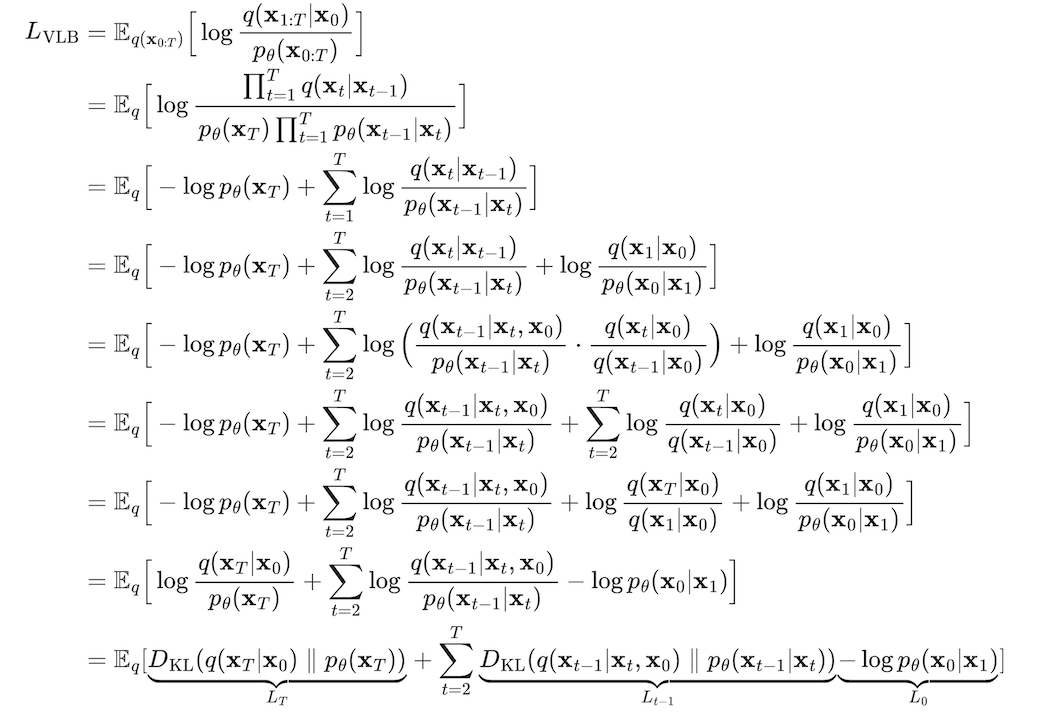
进一步对$L_\text{VLB}$推导，可以得到熵与多个KL散度的累加，推导过程

Untitled

Notes:
- basic knowledge about logarithms:
$$ \begin{aligned} logA + logB = logAB \ logA − logB = logA/B \ logA^n = nlogA \end{aligned} $$
- line 4 → line 5: Markov property of the forward process, and the Bayes’ rule
  
  $$ \begin{aligned} q(x_{t}|x_{t-1}) &= q(x_{t}|x_{t-1}, x_0) \ \end{aligned} \ P(A \mid B,C) = \frac{P(B \mid A,C) ; P(A \mid C)}{P(B \mid C)} $$

也可以写作：

$\begin{aligned} L_\text{VLB} &= L_T + L_{T-1} + \dots + L_0 \\ \text{where } L_T &= D_\text{KL}(q(\mathbf{x}_T \vert \mathbf{x}_0) \parallel p_\theta(\mathbf{x}_T)) \\ L_t &= D_\text{KL}(q(\mathbf{x}_t \vert \mathbf{x}\_{t+1}, \mathbf{x}_0) \parallel p_\theta(\mathbf{x}_t \vert\mathbf{x}\_{t+1})) \text{ for }1 \leq t \leq T-1 \\ L_0 &= - \log p_\theta(\mathbf{x}_0 \vert \mathbf{x}_1) \end{aligned}$

前向$q$没有可学习参数，${x}_T$是纯噪声，$L_T$可以当作是常数项忽略。而$L_t$则可以看做拉近两个高斯分布 $q(\mathbf{x}_{t-1} \vert \mathbf{x}_{t}, \mathbf{x}_0)$和$p_\theta(\mathbf{x}_{t-1} \vert\mathbf{x}_{t})$, 根据多元高斯分布的KL散度求解：

参数化$L_t$

我们需要学习一个神经网络来逼近反向扩散过程中的条件概率分布：$p_\theta(\mathbf{x}_{t-1} \vert \mathbf{x}_t) = \mathcal{N}(\mathbf{x}\_{t-1}; {\mu}_\theta(\mathbf{x}_t, t), {\Sigma}_\theta(\mathbf{x}_t, t))$。我们需要训练一个$\boldsymbol{\mu}_\theta$来预测$\tilde{\boldsymbol{\mu}}_t = \frac{1}{\sqrt{\alpha_t}} \Big( \mathbf{x}_t - \frac{1 - \alpha_t}{\sqrt{1 - \bar{\alpha}_t}} \boldsymbol{\epsilon}_t \Big)$。因为$\mathbf{x}_t$ 在训练时是当作输入参数，我们可以重新参数化高斯噪声项，以使其根据 timestep $t$的输入$x_t$来预测${\epsilon}_t$：

$\begin{aligned} {\mu}_\theta(\mathbf{x}_t, t) &= \color{cyan}{\frac{1}{\sqrt{\alpha_t}} \Big( \mathbf{x}_t - \frac{1 - \alpha_t}{\sqrt{1 - \bar{\alpha}_t}} \boldsymbol{\epsilon}_\theta(\mathbf{x}_t, t) \Big)} \\ \text{Thus }\mathbf{x}_{t-1} &= \mathcal{N}(\mathbf{x}_{t-1}; \frac{1}{\sqrt{\alpha_t}} \Big( \mathbf{x}_t - \frac{1 - \alpha_t}{\sqrt{1 - \bar{\alpha}t}} {\epsilon}_\theta(\mathbf{x}_t, t) \Big), {\Sigma}_\theta(\mathbf{x}_t, t)) \end{aligned}$

The loss term $L_t$

$\begin{aligned} L_t &= \mathbb{E}_{\mathbf{x}_0, {\epsilon}} \Big[\frac{1}{2 | {\Sigma}_\theta(\mathbf{x}_t, t) |^2_2} | \color{blue}{\tilde{{\mu}}_t(\mathbf{x}_t, \mathbf{x}_0)} - \color{green}{{\mu}_\theta(\mathbf{x}_t, t)} |^2 \Big] \\ &= \mathbb{E}{\mathbf{x}_0, {\epsilon}} \Big[\frac{1}{2 |{\Sigma}_\theta |^2_2} | \color{blue}{\frac{1}{\sqrt{\alpha_t}} \Big( \mathbf{x}_t - \frac{1 - \alpha_t}{\sqrt{1 - \bar{\alpha}_t}} {\epsilon}_t \Big)} - \color{green}{\frac{1}{\sqrt{\alpha_t}} \Big( \mathbf{x}_t - \frac{1 - \alpha_t}{\sqrt{1 - \bar{\alpha}_t}} {{\epsilon}}_\theta(\mathbf{x}_t, t) \Big)} |^2 \Big] \\ &= \mathbb{E}{\mathbf{x}_0, {\epsilon}} \Big[\frac{ (1 - \alpha_t)^2 }{2 \alpha_t (1 - \bar{\alpha}_t) | {\Sigma}_\theta |^2_2} |{\epsilon}_t - {\epsilon}_\theta(\mathbf{x}_t, t)|^2 \Big] \\ &= \mathbb{E}{\mathbf{x}_0, {\epsilon}} \Big[\frac{ (1 - \alpha_t)^2 }{2 \alpha_t (1 - \bar{\alpha}_t) | {\Sigma}_\theta |^2_2} |{\epsilon}_t - {\epsilon}_\theta(\sqrt{\bar{\alpha}_t}\mathbf{x}_0 + \sqrt{1 - \bar{\alpha}_t}{\epsilon}_t, t)|^2 \Big] \end{aligned}$

简化 $L_t$

$\begin{aligned} L_t^\text{simple} &= \mathbb{E}_{t \sim [1, T], \mathbf{x}_0, \boldsymbol{\epsilon}_t} \Big[|\boldsymbol{\epsilon}_t - \boldsymbol{\epsilon}_\theta(\mathbf{x}_t, t)|^2 \Big] \\ &= \mathbb{E}_{t \sim [1, T], \mathbf{x}_0, \boldsymbol{\epsilon}_t} \Big[|\boldsymbol{\epsilon}_t - \boldsymbol{\epsilon}_\theta(\sqrt{\bar{\alpha}_t}\mathbf{x}_0 + \sqrt{1 - \bar{\alpha}_t}\boldsymbol{\epsilon}_t, t)|^2 \Big] \end{aligned}$

最后的目标函数是：

$L_\text{simple} = L_t^\text{simple} + C$

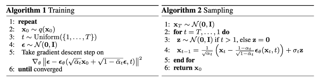
训练过程可以归纳为：

从真实数据分布中随机sample一个 $x_0$, 从$1…T$随机采样一个$t$.
从标准高斯分布采样一个噪声 ${\epsilon}_t\sim {\mathcal {N}}(0 ,I)$
最小化 $\begin{aligned}|{\epsilon}_t - {\epsilon}_\theta(\sqrt{\bar{\alpha}_t}\mathbf{x}_0 + \sqrt{1 - \bar{\alpha}_t}{\epsilon}_t, t)|\end{aligned}$

Untitled

小结

Forward diffusion process: 前向扩散过程，这部分主要是通过重参数化，得到

$$ \begin{aligned} q(\mathbf{x}_t \vert \mathbf{x}_0) &=\mathcal{N}(\mathbf{x}_t; \sqrt{\bar{\alpha}_t} \mathbf{x}_0, (1 - \bar{\alpha}_t)\mathbf{I}) \end{aligned} $$

Reverse diffusion process：反向扩散处理（去噪），这部分主要通过利用贝叶斯公式，利用$x_t, x_0$得到$x_{t-1}$

$$ q(\mathbf{x}_{t-1} \vert \mathbf{x}_t, \mathbf{x}_0) = \mathcal{N}(\mathbf{x}{t-1}; {\tilde{{\mu}}}(\mathbf{x}_t, \mathbf{x}_0), {\tilde{\beta}_t} \mathbf{I}) \\ \begin{aligned} \tilde{{\mu}}_t &={\frac{1}{\sqrt{\alpha_t}} \Big( \mathbf{x}_t - \frac{1 - \alpha_t}{\sqrt{1 - \bar{\alpha}_t}} {\epsilon}_t \Big)} \text{ ;where } {\epsilon}_{t} \sim \mathcal{N}(\mathbf{0}, \mathbf{I})\end{aligned} $$

Diffusion训练，这部分首先利用变分下限来优化负对数似然来得到：

$\begin{aligned} L_\text{VLB} &= L_T + L_{T-1} + \dots + L_0 \\ \text{where } L_t &= D_\text{KL}(q(\mathbf{x}_t \vert \mathbf{x}_{t+1}, \mathbf{x}0) \parallel p_\theta(\mathbf{x}_t \vert\mathbf{x}_{t+1})) \text{ for }1 \leq t \leq T-1 \\ \end{aligned}$

然后利用1，2中的结论代入到$L_t$:

$$\begin{aligned} L_t &= \mathbb{E}_{\mathbf{x}_0, {\epsilon}} \Big[\frac{1}{2 | {\Sigma}\theta(\mathbf{x}_t, t) |^2_2} | \color{blue}{\tilde{{\mu}}_t(\mathbf{x}_t, \mathbf{x}_0)} - \color{green}{{\mu}\theta(\mathbf{x}_t, t)} |^2 \Big] \\ &= \mathbb{E}{\mathbf{x}0, {\epsilon}} \Big[\frac{1}{2 |{\Sigma}\theta |^2_2} | \color{blue}{\frac{1}{\sqrt{\alpha_t}} \Big( \mathbf{x}_t - \frac{1 - \alpha_t}{\sqrt{1 - \bar{\alpha}_t}} {\epsilon}_t \Big)} - \color{green}{\frac{1}{\sqrt{\alpha_t}} \Big( \mathbf{x}_t - \frac{1 - \alpha_t}{\sqrt{1 - \bar{\alpha}t}} {{\epsilon}}\theta(\mathbf{x}_t, t) \Big)} |^2 \Big] \\ &= \mathbb{E}{\mathbf{x}_0, {\epsilon}} \Big[\frac{ (1 - \alpha_t)^2 }{2 \alpha_t (1 - \bar{\alpha}_t) | {\Sigma}\theta |^2_2} |{\epsilon}_t - {\epsilon}_\theta(\mathbf{x}_t, t)|^2 \Big] \\ &= \mathbb{E}{\mathbf{x}_0, {\epsilon}} \Big[\frac{ (1 - \alpha_t)^2 }{2 \alpha_t (1 - \bar{\alpha}_t) | {\Sigma}\theta |^2_2} |{\epsilon}_t - {\epsilon}_\theta(\sqrt{\bar{\alpha}_t}\mathbf{x}_0 + \sqrt{1 - \bar{\alpha}_t}{\epsilon}_t, t)|^2 \Big] \end{aligned}$$

在训练的时候loss为：

\begin{aligned}|{\epsilon}_t - {\epsilon}_\theta(\sqrt{\bar{\alpha}_t}\mathbf{x}_0 + \sqrt{1 - \bar{\alpha}_t}{\epsilon}_t, t)| \end{aligned}

代码部分

Training

def forward(self, x_0):
        """
        Algorithm 1.
        """
        t = torch.randint(self.T, size=(x_0.shape[0],), device=x_0.device)
        noise = torch.randn_like(x_0)
        x_t = (
            extract(self.sqrt_alphas_bar, t, x_0.shape) * x_0
            + extract(self.sqrt_one_minus_alphas_bar, t, x_0.shape) * noise
        )
        loss = F.mse_loss(self.model(x_t, t), noise, reduction="none")
        return loss

Sampling

class GaussianDiffusionSampler(nn.Module):
    def __init__(self, model, beta_1, beta_T, T):
        super().__init__()

        self.model = model
        self.T = T

        self.register_buffer("betas", torch.linspace(beta_1, beta_T, T).double())
        alphas = 1.0 - self.betas
        alphas_bar = torch.cumprod(alphas, dim=0)
        alphas_bar_prev = F.pad(alphas_bar, [1, 0], value=1)[:T]

        self.register_buffer("coeff1", torch.sqrt(1.0 / alphas))
        self.register_buffer(
            "coeff2", self.coeff1 * (1.0 - alphas) / torch.sqrt(1.0 - alphas_bar)
        )

        self.register_buffer(
            "posterior_var", self.betas * (1.0 - alphas_bar_prev) / (1.0 - alphas_bar)
        )

    def predict_xt_prev_mean_from_eps(self, x_t, t, eps):
        assert x_t.shape == eps.shape
        return (
            extract(self.coeff1, t, x_t.shape) * x_t
            - extract(self.coeff2, t, x_t.shape) * eps
        )

    def p_mean_variance(self, x_t, t):
        # below: only log_variance is used in the KL computations
        var = torch.cat([self.posterior_var[1:2], self.betas[1:]])
        var = extract(var, t, x_t.shape)

        eps = self.model(x_t, t)
        xt_prev_mean = self.predict_xt_prev_mean_from_eps(x_t, t, eps=eps)

        return xt_prev_mean, var

    def forward(self, x_T):
        """
        Algorithm 2.
        """
        x_t = x_T
        for time_step in reversed(range(self.T)):
            print(time_step)
            t = (
                x_t.new_ones(
                    [
                        x_T.shape[0],
                    ],
                    dtype=torch.long,
                )
                * time_step
            )
            mean, var = self.p_mean_variance(x_t=x_t, t=t)
            # no noise when t == 0
            if time_step > 0:
                noise = torch.randn_like(x_t)
            else:
                noise = 0
            x_t = mean + torch.sqrt(var) * noise
            assert torch.isnan(x_t).int().sum() == 0, "nan in tensor."
        x_0 = x_t
        return torch.clip(x_0, -1, 1)

Basic Knowledge#

DDPM#

Forward diffusion process#

Reverse diffusion process#

Diffusion训练#

参数化$L_t$#

简化 $L_t$#

小结#

代码部分#

Basic Knowledge

DDPM

Forward diffusion process

Reverse diffusion process

Diffusion训练

参数化$L_t$

简化 $L_t$

小结

代码部分